How to Use Excel for 1st, 2nd, 3rd Order Regression
Use QI Macros Scatter Plot As a Starting Point
A QI Macros user recently called with what looked like a homework assignment. Normally, we don't help students with their homework, but I took a look anyway.
He wanted to know if QI Macros could do 2nd and 3rd order regression on his data.
Since no one has asked me this question in almost 20 years of doing business, I had to Google the answer. The answer is simple.
You can do it in native Excel.
Here Is How to Calculate Second and Third Order Regression
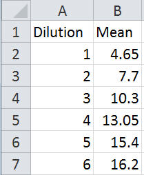
1. Draw a scatter plot of the data. QI Macros scatter plot will automatically give you the first order linear equation. This gives us the first order answers: 2.39 and 2.86:
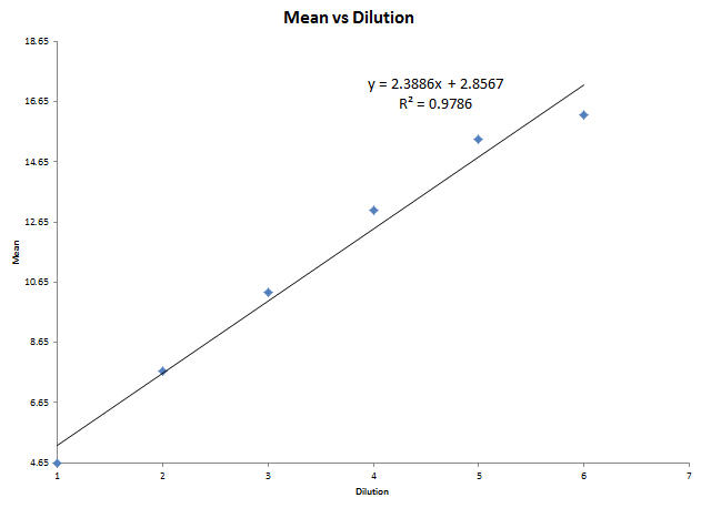
As you can see, the trend line isn't a bad fit (R² = 0.9786), but we can investigate further.
2. Next, right click on the trend line and select Polynomial which gives us the second order answers (-0.22, 3.92, 0.82):
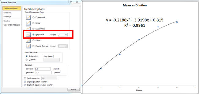
This trend line is a better fit (R2=0.9961).
3. Next, change the Polynomial order to 3 and you get the third order answers (-0.066, 0.476, 1.82, 2.48):
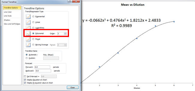
This trend line is a slightly better fit: (R2=0.9989).
Pretty simple, isn't it?
Here's my point:
There's a lot of power hidden in Excel and I keep discovering more every day. Think outside the spreadsheet. What else can you do with Excel?
Other Charts Included in QI Macros for Excel
Join 100,000+ Users
in 80 Countries
![]()